GraphSAGE review
Inductive Representation Learning on Large Graphs, 2017
Summary
-
기존 상황 및 문제점
large graph에서의 노드들의 low-dimensional embeddings 은 유용하나, 많은 방법론들이 embedding 을 학습 시 모든 node들이 존재해야 한다는 단점을 가지고 있다. 이러한 방법론은 transductive 하고 unseen nodes에 대해서 일반화가 되지 않는다는 단점을 가지고 있다. -
본 논문의 제안
이에 본 논문에서는 GraphSAGE 라는 general inductive framework을 제안한다. GraphSAGE 에서는 각 node에 대한 embedding을 학습하기보다는, embedding을 생성할 수 있는 function 을 각 feature embedding을 sampling & aggregating을 통해 학습시킨다. -
실험 결과
본 논문에서는 3 가지의 inductive node classification task에 대해서 타 모델에 비해 outperformance를 달성한다.
Method
본 논문에서 제안하는 바의 key idea는 node의 local neighborhood로부터 feature information 을 어떻게 aggregate 할 수 있을 것인지에 관한 부분이다. 따라서 embedding을 어떻게 generation 할 수 있는지, 그 다음 embedding을 어떻게 학습할 수 있는지에 대해 살펴보자.
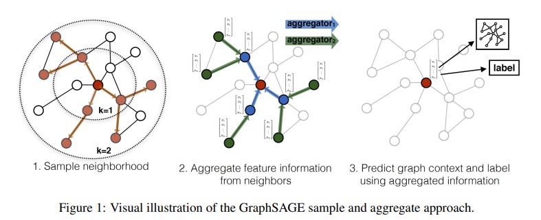
위의 Figure1은 GraphSAGE가 sampling과 aggregate을 통해 node embedding을 학습하는 과정을 시각화한 예시를 보여준다. 각 노드를 기준으로 fixed-size set of neighbors 에 대해서 uniform sampling 을 통해 주변의 이웃들을 sampling 해준다. sampling된 주변의 node embedding을 aggregate 해주고, 자기 자신의 node embedding과 정보를 concat하여 node embedding이 업데이트 된다. 자세한 내용은 아래의 과정에서 살펴보자.
- Embedding generation (i.e., forward propagation) algorithm
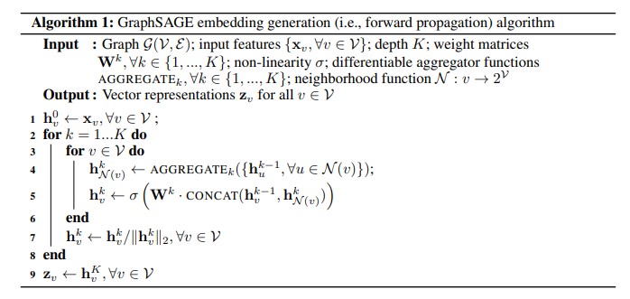
- Embedding은 위의 Algorithm 과 같은 방식으로 생성된다. 주요한 line들에 대해 작동하는 방식을 살펴보면 아래와 같다.
- line 4: k-1 layer에 있는 feature embedding h에서 neighborhood function 에 속해 있는 u node들에 대해 aggregate function 을 통해 neighborhood embedding $h_{N(v)}^k$를 얻어준다.
- line 5: 업데이트 대상이 되는 v node의 h embedding과 concat 을 해준 후, k layer의 weight matrix W를 곱해주어 새로운 embedding을 얻는다. 이후 nonlinear activation function 을 취해 $h_v^k$를 얻는다.
- line 7: hyperspere normalization을 취해 준다. 이렇게 normalization을 취해주면 NNS(Nearest Neighbor Search)에 유용하다고 하다.
- Relation to the Weisfeiler-Lehman Isomorphism Test
위의 Algorithm 1은 the Weisfeiler-Lehman (WL) isomorphism test(also known as “naive vertex refinement”) 의 하나의 instance 가 될 수 있다. (WL isomorphism 에서 isomorphic 이란 subgrah A에서 edge 로 이웃한 모든 node 들의 쌍에 대해, subgraph B에서 대응되는 각 node 들의 쌍 또한 edge 로 이웃해 있을 때 isomorphic 하다고 한다.) 2개의 subgraph 에 대해서 Algorithm 1의 output 이 identical 하면, WL test 는 두 그래프를 identical 하다고 말한다. GraphSAGE는 large graph의 representaion 을 학습하기 위한 model 이지만, WL test에 continuous approximation 을 하기도 한다.
- Embedding은 위의 Algorithm 과 같은 방식으로 생성된다. 주요한 line들에 대해 작동하는 방식을 살펴보면 아래와 같다.
-
Learning the parameters of GraphSAGE
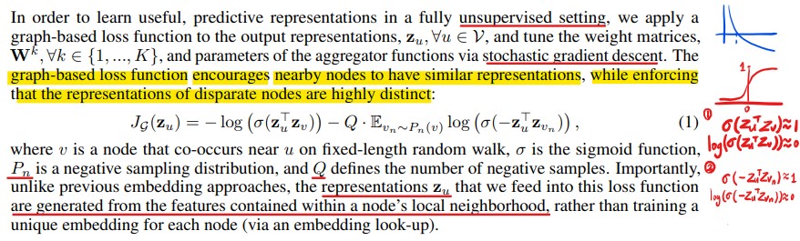
GraphSAGE는 unsupervised learning 학습하는 방법을 제안한다. 위와 같은 수식으로 학습이 되며, 간단하게 이야기하면, output representation z에 대해서 positive smaple사이의 embedding은 서로 유사한 값을 가지게 하며, negative sample사이의 embedding에 대해서는 서로 다른 값을 가지게 하는 식으로 학습된다. 이를 통해 positive sample과는 더욱 가까워지고, negative sample과는 더욱 멀어지게 된다. 여기서 positive sample은 fixed-length random walk을 수행하여 얻어진 sample(uniform sampling)을 이용하고, negative sample은 large graph이기 때문에 여기서는 random sampling을 수행하면 높은 확률로 negative sample이 selection된다. -
Aggregator Architecture
다른 N-D lattices 꼴의 data modality와 달리, node의 이웃들 사이에는 natural ordering이 없다. 따라서 Aggregator function도 unordered vector set에 대해서 작동하는 것이 합리적이다. 이에 Aggregator function은 input의 permutation에 invariant 하기 위해서 symmetric한 특성을 가지는 것이 이상적이다. 본 논문에서는 아래와 같은 3가지 타입의 Aggregator function을 활용한다.-
Mean Aggregator

Mean Aggregator에서는 neighborhood representation vector 와 자신의 representaion vector에 대해서 elementwise mean을 수행한다. 위의 Algorithm 1에서 line4,5번이 위의 수식으로 대체되어 수행된다. 논문에서는 이러한 modified mean-based aggregator “convolutional”하다고 한다. 그 이유는 rough하게 localized spectral convolution의 linear approximation으로 볼 수 있기 때문이다.
-
LSTM Aggregator
LSTM Aggregator는 symmetric한 특성을 가진 function은 아니다. 잘 알려져있다 시피, LSTM은 sequential input data에 대해 주로 사용된다. 한편, 여기에서는 input nodes(node’s neighborhood)를 random permutation을 수행하였고, 이를 input으로 순차적으로 주었다. 놀랍게도, mean aggregator에 비해 larger expressive capability를 가진다. -
Pooling Aggregator
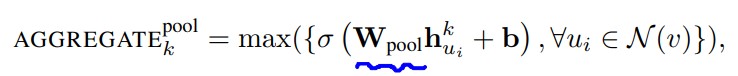
Pooling aggregator는 symmetric & trainable하다. 해당 방법론에서는 각각의 neighbor’s vector가 독립적으로 FC layer를 거치고 elementwise max-pooling이 적용되는 방식이다. 각각의 계산된 feature에 max pooling oeprator를 적용하여, neighborhood 집합의 각기 다른 면을 효과적으로 capture할 수 있다.
-
Experiments
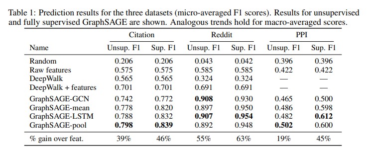
본 논문에서의 실험은 3개의 dataset에 대해 node classification을 수행한 결과를 보여준다.
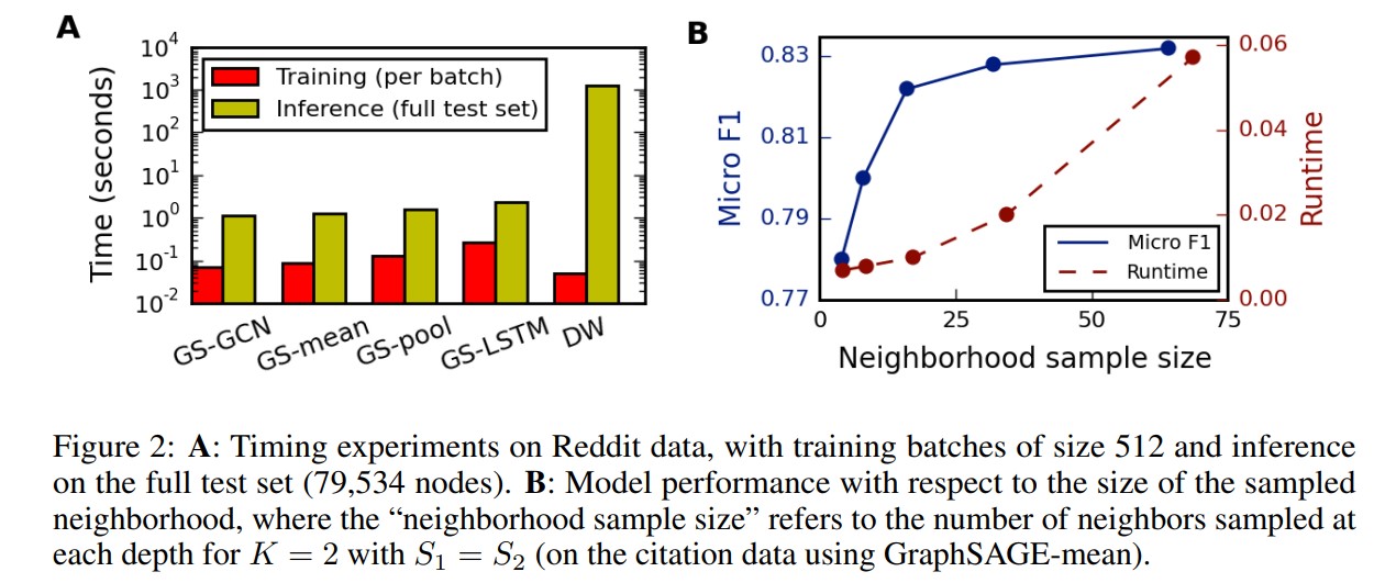
위의 그림에서는 large scale 그래프에 대해서 GraphSAGE의 시간대비 효율성을 보여준다. 왼쪽의 A에서는 GraphSAGE 모델이 transductive한 Deep Walk 모델에 비해서 inference time이 얼마나 감소되는지를 보여준다. 오른쪽의 B에서는 Neighborhood를 얼마나 sampling하냐에 따라 F1-score, Runtime의 변화를 보여주고 있다.
Reference
느낀 점
- random permutation 을 수행한 LSTM aggregator function이 좋은 성능을 보인 것이 흥미로웠다.
- MHSA(Multi Head Self Attention) aggregator function 을 활용하면 어떤 결과가 나올지 궁금하다.
- multi head를 이용하는 점, self-attention 이 inductive bias가 약한 점을 고려하면 더 다양한 관점의 feature를 내포할 수 있지 않을까?