Probability 기초 정리
probability & random vairable 기초 내용을 정리합니다.
Elements of probability
- sample space
- set of outcomes
- probability measures
- event 가 입력으로 들어왔을 떄 거기에 대응되는 함수
- 몇몇 properites
Random Variables
- Probability Measure for Random Variable
- CDF
- culmulative
- culmulative
- PMF (Mass Function)
- discrete 한 경우
- discrete 한 경우
- PDF (Density Function)
- continuous 한 경우
- density function 의 prob 자체는 매우 큰 무한대까지 가질 수 있음. 왜냐면, x의 범위가 어어어어엄청 0에 가깝게 작아지면, 적분하면 1이 되어야 해서.
- 어떤 RV x 에서 어떤 RV y 에 대한 분포를 transformation 해서 구한다고 생각해보자.
y = f(x) 일 때, P_y(y) = P_x(x)*|gradient| 로 구해짐.
일반적으로 vector의 경우도 그러함. 여기서 f를 NN 으로 쓰게 되면, invertible 하지 않기 때문에 y의 likelihood 를 구할 수가 없음. - Normalizing Flow
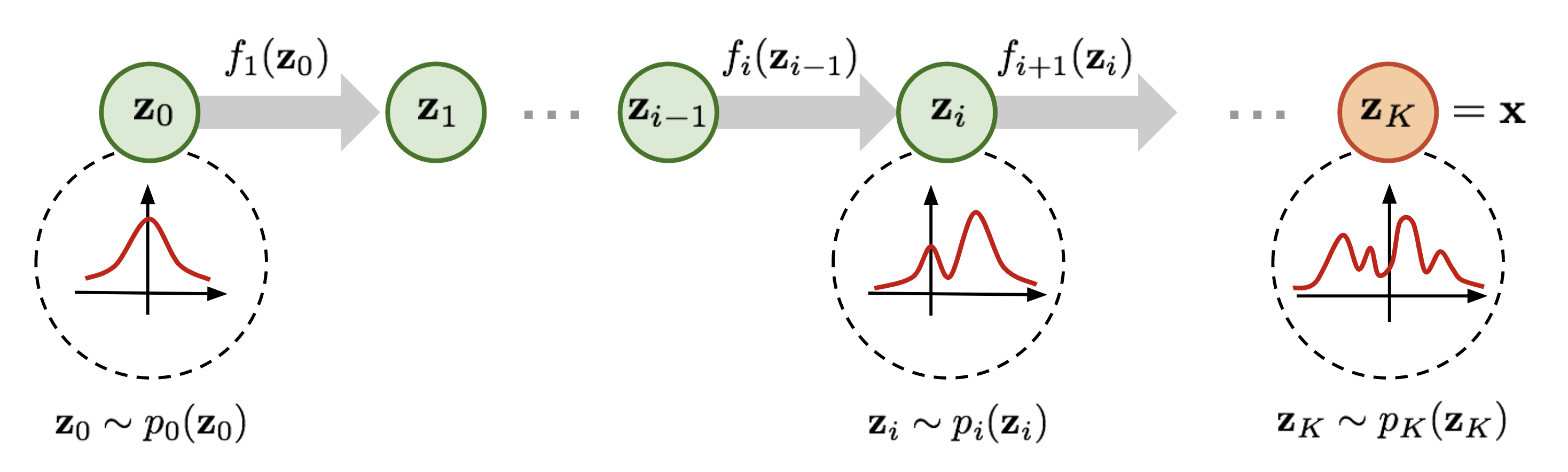
Normalizing Flwo는 invertible transformation 을 통해 점점 좀 더 복잡한 distritbuiton 을 invertible한 연산을 통해 만들어 나간다.
이를 통해 최종 target variable의 probability distribution을 invertible transformation을 통해 추적할 수 있다. - Masked Autoregressive Flow
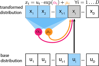
각 step을 거치며 지나는 분포를 NN의 invertible 함에서 얻는 것이 아니라, NN의 autoregressive 함을 통해 각 step의 평균과 분산을 얻는다.
base distribution을 정보와 이전 스텝의 평균, 분산 정보를 활용하여 해당 step i의 x_i 값을 구한다. - Inverse Augoregressive Flow
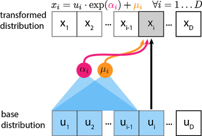
위의 MAF 는 sampling 과정의 속도가 heavy해서, 평균과 분산을 얻는 것을 base distribution 에서 뽑아보자는 제안
- continuous 한 경우
- CDF
- Expectation & Variance
- Expectation 은,, E[X] = sum(p_x*x) 임
- Distrete Distribution
- Bernoulli (Binary Distribution)
- p(x) = p^x*(1-p)^(1-x)
- Binomial
- binary distribution 이 N번 수행되는 것
- Negative Binomial
- n 번의 failure 가 observable 할 때까지 몇 개의 1이 등장하는지 무한해질 수 있음
- Poisson
- event 의 발생 횟수가 궁금할 때
- Bernoulli (Binary Distribution)
- Continuous Distribution
- Normal (CLT, useful in many domains) / Uniforam / Exponential
- 어떤 distribution이 있는지 아는 것보다, 내가 사용하고자 하는 random variable 이 어떤 distribution에 mapping 되는지 인지하는 것이 더 중요함!
- Variance
- 평균으로부터 퍼져있는 정도
- multiple variable 가 될 경우
- joint distribution으로 표현할 수 있음
- joint distribution 의 상대적으로 대조되는 개념은 marginal distribution!
- marginal은 여러 다 변수 중 1,2개의 변수만을 고려하는 경우, 즉 그 1,2개의 변수만을 marginalized 시키는 경우이다.
- Indepence
- cdf, pdf, pmf 등에서 joint distribution이 각 random variable의 distribution으로 factorization 이 되면 독립이라고 말할 수 있음
- Convariance
- 두개 이상의 변수 사이의 퍼짐 정도. (variation의 extension)
- 만약 두 변수가 independent 하다면, uncorrelated 하다고 말할 수 있음 (역은 성립 못함)
- Correlation
- Normalized version of covarriance 이다
- corr[X,Y] = Cov[X,Y] / sqrt(Var(X), Var(Y)) (-1과 1 사이의 값)
- Covariance Matrix
- multiple variables 일 경우, Covariance 값을 각 변수 사이에 따라 matrix로 표현 가능
- Multivariate Normal Distribution
- Normal Distribution을 1변수에서 다변수로 자연스럽게 확장할 수 있음 scalar → vector
- 매우 유용함
- MLE(Maximum Likelihood Estimation) interpolation for least square
- Gaussian Mixtutre Model
- 여러가지의 Gaussian Dist component 들을 합성하는 방법론
- Even in Bayesian DL (Gaussian Prior)
- prior distribution을 가정하는 경우에도 많이 쓰임
- 기억하기 !
- joint distribution 이 normal 이면 marginal distribution도 normal 이다!
- joint distribution 이 normal 이면 conditional distribution 도 normal이다!
- 다소 복잡한(?) 값을 과정과 값을 가지지만, Schur complement 에 의해 Precision Matrix (Covariance의 Inverse Matrix) 의 값을 활용하여 계산하면, normal distribution 이 됨을 보일 수 있음
2 RULES! (Important)
- conditinal probabiltiy
- 일반적으로 딥러닝은, 기존의 데이터 X 가 주어질 때 , 새로운 보지 않은 데이터 X’ 가 나올 확률을 구하는 문제이다. 따라서 조건부 확률적인 부분이 중요하다.
\(P_{Y|X}(y|x) = \frac{P_{X,Y}(x,y)}{P_X(x)}\) - 즉, conditional probability 는 “x가 이미 발생한 이후, joint distritbution 이 발생한 경우” 로 볼 수 있음
- 참고
- joint distribution P(X,Y)
어떤 사건 X,Y가 동시에 일어나는 확률 분포 - conditional distribution P(X|Y)
사건 Y가 일어났을 때, 사건 X 가 일어날 확률 분포 - marginal distribution P(X) or P(Y)
joint distribution 이 다변수를 고려한다면, 그 중 하나의 변수를 고려할 때, “marginalized 되었다” 라고 표현한다.
하나의 변수는 상수 취급하고, 하나의 변수만 취급하는 식으로 더 적은 변수들만 고려하는 경우
(다변수에서 상대적으로 더 적은 변수를 고려할 때)
- joint distribution P(X,Y)
- 일반적으로 딥러닝은, 기존의 데이터 X 가 주어질 때 , 새로운 보지 않은 데이터 X’ 가 나올 확률을 구하는 문제이다. 따라서 조건부 확률적인 부분이 중요하다.
- sum rule
- P(x) = sum(P(x,y)) (y에대해 summation 할 때)
- joint prob p(x,y) 를 y 또는 x 하나의 변수에 대해서 summation하면 marginal distribution을 얻을 수 있음.
- joint prob p(x,y) 를 y 또는 x 하나의 변수에 대해서 summation하면 marginal distribution을 얻을 수 있음.
- continuous 한 경우는 integral 을 써서 보이면 됨.
- P(x) = sum(P(x,y)) (y에대해 summation 할 때)
- product rule
- joint distribution = conditional distribution * marginal distribution 이 됨.
- P(X,Y)
= P(Y|X) * P(X)
= P(X|Y) * P(Y) - Example
marginal prob P(Y_o)
= P(Y_o, X_red) + P(Y_o, X_blue)
= summation of {joint distribution}
(joint dist. 은 product rule로 conditional dist. * marginal dist. 로 표현 가능)
= P(Y_o|X_red) * P(X_red) + P(Y_o|X_blue) * P(X_blue)
(각 joint distribution = product rule 로 값을 표현할 수 있음)
so,
= product rule_1 + product_rule_2
(이 값들은 구할 수 있는 경우 有) - opinion) joint distribution을 conditional dist. 와 좀 더 적은 변수를 고려하는 marginal dist.로 분해할 수 있는 product rule이 꽤나 유용한 거 같음
- joint distribution = conditional distribution * marginal distribution 이 됨.
Self 문답
-
implicit 의 의미는?
내가 이해한 바로는, y의 pdf는 얻을 수가 없다는 말이다. 왜냐하면, y로 가는 함수 f 자체가 direct 하게 distribution을 approximation 하려 하는 것인데, 이 f가 invertible 하지 않기 때문이다. -
그래서 invertible한 tranformation 을 가지는 연구 흐름이 normalizing flow이다.
affine transfomration, leakly ReLu 등 invertible 한 변환들을 활용하여, gradient 를 trackable하게 구하고, 기존 x 에서, y로 변환되는 부분들을 얻고자 하는 것이다. -
likelihood (가능도 즉, 어떤 결과 x가 관찰되었을 때, 그 결과가 나올 확률 분포 distribution이 얼마인지 예측하는 값)
참고 링크 : https://jjangjjong.tistory.com/41
Reference
- https://blog.evjang.com/2018/01/nf2.html
- https://lilianweng.github.io/posts/2018-10-13-flow-models/
- https://jjangjjong.tistory.com/41